| Email: info@psq.co.za Phone: 021 557 2491 Subscribe to our Newsletters |
| |
| Newsletter |
Lead Times in Supply Chain
by Bernard Milian 
Implicitly,
when we think of pull flow, Kanban for example, we think of short lead
time. Consumption triggers the next supply, so this implies a
rapid reaction time, doesn’t it?
On the other hand, for components with long lead times – say for example, an item with a replenishment lead time of 4 months / 16 weeks – we’ll consider the projected requirements derived from our sales forecasts via the master production schedule, week by week, for the next 16 weeks and more. This will enable us to determine when the next replenishment should arrive. We tend to believe that making the right replenishment decision requires a detailed analysis of the forecasts and their timing, week by week.
Kanban is OK for short lead times, but beyond that, for long lead times, we need MRP (Materials Requirement Planning) – this logic is engraved in our minds, isn’t it?
Renewing consumption
Let’s return to the basic principle of a pull flow. It’s all about renewing consumption. Whether it takes four days or four months, this logic remains valid. Given what I consume, I need to trigger a complementary supply flow. So if my supplier lead time is 4 months, I need to trigger a replenishment that will arrive in four months.
We are in the same logic of refilling a loop.
A longer loop
It’s just that the loop is longer. In DDMRP
(Demand Driven Materials Requirement Planning) terms, the top of the
green zone will represent a higher number of days, and the yellow zone
will be of greater proportion.
In the examples below, the item on the left has a lead time of 7 days, and the item on the right is 150 days.

In the examples below, the item on the left has a lead time of 7 days, and the item on the right is 150 days.
The replenishment principle is the same; if my net flow equation falls below the top of yellow, I have to trigger a complementary flow.
Planning and Execution
Let’s
face it; in 150 days, more is going to happen than in 7 days. To
establish our buffer and calculate the reorder point that is the top of
the yellow zone, we calculate an average future consumption over the
next 150 days – which is what our yellow zone represents.
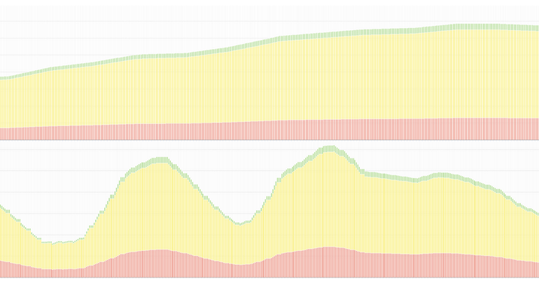
For example, if we compare the forecasts of the two items below, which have the same long lead time, over the next 12 months, we’ll need to keep a closer eye on the timing of the second item, as demand is more volatile. These two items may have the same average daily forecast as of now and therefore the same yellow zone.
For example, if we compare the forecasts of the two items below, which have the same long lead time, over the next 12 months, we’ll need to keep a closer eye on the timing of the second item, as demand is more volatile. These two items may have the same average daily forecast as of now and therefore the same yellow zone.
While in the case of a short lead time, planning and execution are closely related or even merged, in the case of a long lead time we need to pay more attention to execution. Generating an order follows the same logic, but we’ll need to make sure that the goods arrive on time, while actual consumption is likely to differ from forecasts every week.
With a long lead time, there is more distance between the moment when an order is generated (planning) and its availability in stock (execution) – so we need to focus more on the latter. The timing of demand over the next 150 days, and actual consumption, will have to be monitored – and action taken by exception.
MRP is no better than pull flow for long lead times – it may give the impression of greater precision, as orders are triggered based on the projected stock based on each week’s forecasts – but this is an illusory precision, since the reality will be different.
Improving visibility
Experience
shows that the practice of pull flow on long lead items leads gradually
to better stock balancing – improved service, reduced
overstocking – thanks in particular to greater visibility, and
less variability in order generation.
The MRP logic also often leads planners into firming up orders too early, well beyond the item’s actual lead time – which amplifies the bullwhip effect. Pull flow encourages decisions to be taken at the right moment, neither too early nor too late.
However, there is no magic. Long lead times imply greater inertia, higher capital requirements, greater risks, and more resources to monitor execution. Shortening lead times through better supply chain design, shorter distances, and intermediate decoupling points, remains the best solution.
Get in touch.
For more information, contact KenTitmuss.
About the Author
Bernard Milian has more than 35 years of experience in developing agility within industrial and distribution supply chains. He has more than 25 years of experience in Supply Chain Management and Continuous Improvement / Lean 6 Sigma transformation. He has served as a Supply Chain Director within French subsidiaries of world class corporations, in the automotive, electronics, medical devices, furniture and metallurgy industries, B2B, B2C, manufacturing and distribution environments
Bernard Milian has more than 35 years of experience in developing agility within industrial and distribution supply chains. He has more than 25 years of experience in Supply Chain Management and Continuous Improvement / Lean 6 Sigma transformation. He has served as a Supply Chain Director within French subsidiaries of world class corporations, in the automotive, electronics, medical devices, furniture and metallurgy industries, B2B, B2C, manufacturing and distribution environments